Contents
Description
- This example begins with a simple 2D, one-element mesh with sharp corners. The element corners are made smooth and continuous by defining higher-order Cubic Hermite basis functions and adjusting their derivatives appropriately. The purpose of this exercise is to further explore the meaning of the derivatives that function as nodal parameters for the higher-order basis functions within Continuity.
-
The files needed for this exercise can be found in the Continuity Tutorials folder (if you have downloaded it) under Mesh -> exercise3. The cont6 file containing the entire problem setup can also be downloaded by clicking here.
Basic Concepts
- After completing the Mesh module tutorials 1 and 2, you should understand that:
- Each node has several parameters associated with it.
- The number of associated parameters depends on the type of basis function(s) in use
- Elements are defined by specifying connections between nodes
- Nodal parameters determine the shape of an element, including the location of its corners and the shape of its edges, surfaces, and volume
-
After completing this tutorial, you should understand:
- The practical meaning of first-order nodal derivatives
- How to perform simple manipulations of nodal derivatives, such as:
- Using Continuity to calculate some derivatives automatically
- Relating nodal derivatives to each other to achieve smooth, continuous mesh boundaries
- Useful points to consider:
- While analytically determining the correct values for nodal derivatives can be daunting, the good news is that with care Continuity can be made to do most of the work for you.
- When it comes to creating detailed, anatomically realistic meshes, manually adjusting derivative values to fit a data set would be enormously difficult, and in practice is never done. Instead, after defining some simple constraints on nodal parameters (the basics of which you learn in this tutorial), Continuity’s Fitting module does the job of adjusting mesh parameters in an automated way.
Step-by-step Instructions
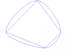
- The following instructions will guide you in creating the mesh pictured below and then lead you through altering it to make a smooth, continuous shape.
Start Continuity
- Launch the Continuity 6.3 Client
-
On the About Continuity 6.3 startup screen
-
check the mesh box under Use Modules:
-
Create Mesh
-
-
Select rectangular cartesian in the Global Coordinates: pop-up menu
-
Click OK to submit Coordinate Form
-
-
-
Choose Lagrange Basis Function→2D→Linear-Linear with 3 integration/collocation points for Xi 1, Xi 2, and Xi 3
-
Click Add
-
Choose Hermite Basis Function→2D→Cubic-Cubic with 3 integration/collocation points for Xi 1, Xi 2, and Xi 3
-
Click Add
-
Click OK to submit Basis Form
-
-
-
Click Import/Export/Graph button to open Continuity Table Manager
-
Continuity Table Manager→File→Open…
-
Select tab-delimited nodes file nodes.xls
-
-
-
Note that Linear-Linear Lagrange 3*3 is already selected for you under Coordinate 1, Coordinate 2, and Coordinate 3
-
Note also that all derivative values are currently set to zero. We need to obtain correct derivative values before being able to use the higher-order bicubic Hermite basis functions.
-
Click OK to submit Node Form
-
-
-
In this case, the element definition is simply 1, 2, 3, 4, so enter this in the Global Node Numbers box
-
Click OK to submit Element Form
-
-
-
Click the lines radio button
-
Click Render to display mesh
-
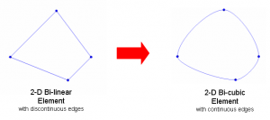
Convert from Linear-Linear to Cubic-Cubic
- Switching to cubic Hermite basis functions requires the determination of 3 new parameters per coordinate direction per node. In this case, that’s a total of 24 parameters. Rather than trying to manually determine the values of these parameters, we can use Continuity’s Refine feature. Because we have defined a cubic-cubic Hermite basis function, upon doing a 1 by 1 refine the necessary derivative values will be calculated and placed in the nodes form.
-
-
Enter 1 for the xi1, xi2, and xi3 fields under New Element per old element in
-
Click OK to submit
-
-
- Note that derivative values are no longer zero
-
Select Cubic-Cubic Hermite 3*3 under Coordinate 1, Coordinate 2, and Coordinate 3
-
Click OK to submit Node Form
- At this point we need to re-send, calculate, and render the mesh:
-
-
Click the lines radio button
-
Click Render to display mesh
-
-
Note that the mesh looks exactly the same. Once again, this is because during the refine 1 by 1 by 1 step, Continuity has calculated the derivative values such that the lines connecting nodes are straight.
Alter Derivatives to Give Smooth Edges
- Suppose we want this element to have smooth, continuous edges (in the global sense). Suppose in particular that we’d like:
-
The element edges at nodes 1 and 4 to be tangent to the x2 axis
-
The element edges at nodes 2 and 3 to be tangent to the x1 axis
-
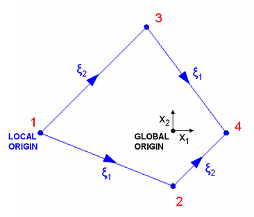
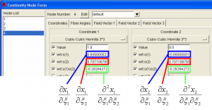
- To understand how to alter the derivatives to achieve these conditions, consider the significance of the nodes form boxes in mathematical notation:
- Consider node 1.
-
In order to make the element edges tangent to the x2 (vertical) axis, moving from node 1 in either the ξ1 or ξ2 direction should produce no change in the x1 direction. In other words,
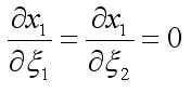
-
Open the nodes form (Mesh→Edit→Nodes…)
-
Click on node 1, and change the appropriate derivative values to zero as described above. Leave all other derivative values as they are for now.
- Now consider each of the other three nodes in turn. Carefully select which pair of derivatives should be set to zero for each node in order to create our desired tangent relationships.
-
Click OK when finished to submit the nodes form.
-
-
Increase the number of divisions from 10 to 25 (View→Set Divisions…)
-
-
Click the lines radio button
-
Click Render to display mesh
-
-
If you have made the changes correctly, the new and old meshes are now superimposed and should look like the picture below. A cont6 file containing the correct derivative values can be found here.