Tutorial on mesh construction from Ultra Sound Images

This tutorial will explain the process of creating ‘new topology’ meshes to be used in Continuity from 2D echocardiographic images.

Contents

Tutorial on mesh construction from Ultra Sound Images

Some general advise

This goes without saying, but save your work often and preferably across different files, so you can always easily go back a step if something goes wrong.

Review the mesh module, mesh generation and Segmentation/Mesh generation tutorials in the continuity documentation to become familiar with using Continuity & Blender.

In Continuity, go to view>edit dimensions after each refinement operation and press ‘apply marked recommendations’. If you run into any errors while running Continuity, faulty dimensions will often be the cause.

Description

These step-by-step instructions will guide you through the process of creating ‘new topology’ meshes to be used in Continuity from 2D echocardiographic images. A zip-file containing example files can be downloaded here: US_mesh_tutorial_files.zip

Software

The software needed to follow the instructions in this tutorial consists of:

synedra view personal
a (simple) image editor like MS paint or paint.NET
ImageJ
Blender 2.49b
Continuity
Matlab (no older than v. 2008b)
notepad and/or excel (to modify .off/tsv files)

Data extraction

Using the program ‘synedra view personal’ open the echo movie files. You can do this by starting the program and dragging your echo files to the document tree on the left side of the screen.
Look for the 4-chamber view and 2 chamber view.
Go to movie view (right upper corner)
In both clips, find the frame that corresponds to the End Diastolic state. The ventricles will be at their largest. It should correspond approximately with the top of the R-peak in the QRS-wave signal.
Right click on the selected movie in the document tree on the left and select ‘convert to JPEG’ and save the image file.
Use a simple image editor (e.g. paint/paint.NET) to remove any sensitive patient data (such as name, dates, ect.).
Open ImageJ and import the image. Use the selection tool to manually trace the contours of the left ventricle (LV), right ventricle (RV), epicardium (EPI) and scale (right hand side of the image).
Interpolate (smooth) selection (Edit>Selection) and export xy-coordinates (File>Save as…). For the 2-chamber view, RV can’t be selected, so of course it doesn’t have to be exported for this view. (Hint: looking at the moving images can really help identifying the outlines of the ventricles)

Data Extraction: Example

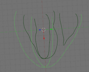
Extraction of xy-coordinates from End Diastolic US images

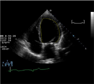
Shown here: Left Ventricle in 4 chamber view

Data Alignment

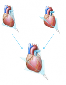
For the alignment of the data, we assume that both views are approximately perpendicular to each other:

Open your coordinate files in a text editor or excel and add 2 lines at the top, the first of which contains the file type: ‘off’ and the second of which contains the total amount of coordinates (i.e. column length of the original file) above the first column and zeros above the other two. The file can now be imported into Blender
Open Blender 2.49b and go to File>import>DEC Object File Format (.OFF)… and select the coordinate file. You probably need to zoom out to see the data.
In object mode, select the objects that belong to the same view and use ‘CTRL + J’ to join the selected meshes. This way the relative position of each component won’t change.
Scale the data according to the scale you extracted from the echo image. The distance between each dot on the scale should be 1 cm. From the scale coordinates the scale factors can be calculated. Select the data and go to view properties (in the view menu). Here you can input the scale factors you calculated.
Press ‘SHIFT + C’, ‘C’ to center the cursor and camera. Select your objects and click object>transform>obdata to center, to center you’re objects.
Now rotate your lateral (2-Chamber) LV object 90 degrees so it is perpendicular to the 4-Chamber view. Use the apex thickness as a guide when aligning the data. Make sure you double check to see if the posterior side of your LV data really is on the posterior side of the heart.
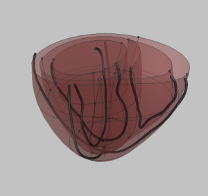
Import the generic prolate mesh into Blender (BiV4_echo.blend).
Select all your data objects and align them with the mesh. Use the apex as a easy anatomical landmark for alignment.
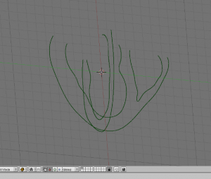
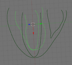
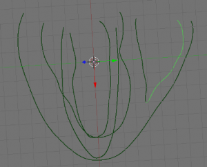
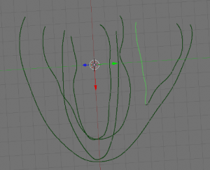
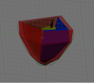
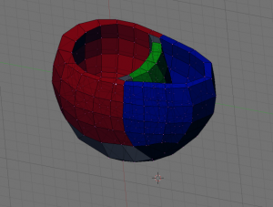
Next, create 4 new objects to be labeled later on, by going into edit mode and selecting the appropriate parts (LV, RV, EPI and septum (ST)) of your data and using ‘SHIFT + D’, ‘ENTER’, ‘P’, ‘ENTER’. Examples shown below: EPI (upper left), LV (upper right), RV (lower left), ST (lower right) highlighted in green.

Export each object as a separate .OFF file. (File>export)
Use the MATLAB script ‘LabelData2ContinuityFormat.m’ to label the data and convert them to a format usable by Continuity. Do this for all 4 data files. (script: LabelData2continuityFormat.m )
Use the MATALB script ‘ConcatenateDataForms.m’ to concatenate the labeled data files into 1 file to import in Continuity. (script: ConcatenateDataForms.m )

Prefitting a simple generic prolate mesh

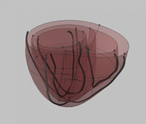
Manually fit prolate mesh to data by moving the nodes around in Blender. This will require some practice since you’ll have to guess where the rendered surfaces will end up (they should run through your data). NB: don’t move the groups of 4 nodes at the apex separately and only move them along the z-axis.
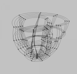
When you think you have a good fit, export the mesh as a .off file
Use the MATLAB script ‘Cartesian2Prolate.m’ to convert the cartesian mesh coordinates to prolate spheroidal coordinates for Continuity to use. (script: catesian2prolate.m)
Load a prolate model into Continuitiy and substitute the node form and data form with your own.
Render the results and repeat steps 1-4 until you’re satisfied with the result.

Fitting the prolate mesh

Use the python script ‘FitGeometry.py’ to perform an automated iterative fit of the prolate mesh surfaces to the data. (script: FitGeometry.py)

View Menu

Refine your fitted prolate mesh using the ‘RefineRenode.py’ python script. This is the mesh used for biomechanics simulations. (script: RefineRenode.py )
Convert the resulting ‘old topology mesh’ to the new topology used for the electro-physiology meshes, using the ‘!Echo128MeshToEP132Mesh.py’ python script. (script: Echo128MeshToEP132Mesh.py )
Open a new Blender file.
Import the .pickle files of you model (one with 280 nodes, one with 26952 nodes) using the HexBlender scripts (scripts>mesh>hexblender…>import pickledhex).
Using the ‘retopo’ function, project the 280 nodes onto their corresponding surfaces of the fine mesh.
Use ‘show edge lengths’ (found in object window, <F7>) to evenly space nodes placed along edges. The best order to work in here is starting with the septum (LV side) > septum (RV side) > RV > apex (inside) > LV > EPI.
Select the surface of the elements you want to regularize and click the ‘regularize surface’ button (hexblender scripts). The nodes on the edge of the selected surface will remain in place (which is why the previous step is necessary). NB: the script will crash if the elements don’t form a rectangle, i.e. the number of elements along each ‘column’ of the surface should be equal.
When you’re done, duplicate you mesh (in object mode, select the mesh and press ‘SHIFT + D’, ‘ENTER’).
Set the number of iterations below ‘TriCubic Hermite’ to 3 and click ‘TriCubic Hermite’. Blender will now refine the mesh and calculate the derivatives. Save them as a .txt file.
Select your unrefined mesh again and use ‘Hex-Keys’ and ‘Conti Vertex’ to export the element and nodes forms, respectively.
Open Continuity and create the model (define coordinates, basis functions (tricubic hermite), nodes (file you just created), elements (idem dito), and scale factors (derivatives file you just calculated).
Send all, calculate mesh, render surfaces (optional).
Under mesh>list> select ‘scaled jacobian’. Save the list.
Open it in Excel and for each element check the minimum Gauss point value. If it lies below the threshold of 0.6, note the element number and go back to your mesh in Blender to improve the element shape. The more skewed the element is, the lower it’s Gauss point values.
Repeat steps 8 – 14 until the mesh quality is satisfactory
Use mesh>refine extraordinary to refine the mesh. Do this twice. (Remember to edit dimensions!)
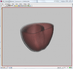
You now have your final mesh.