Description
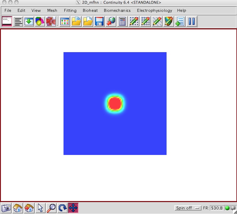
- This example simulates action potential propagation across a 4 mm by 5 mm piece of tissue.
- A 50 mA stimulus with user-defined start time and duration parameters is applied along the center of the tissue. The start time and duration may be altered by the user in the stimulus form. The stimulus strength can be altered in the node form.
- This simulation will make use of the MFHN Ionic model, so we need to load and compile that model.
- Connect to the database from File→Library→Search
-
At the top of the search form search for a Title containing mfhn
-
Right-click on EP_MFHN_sympy and select Load
-
You will get a warning window, select Reset (without save) then proceed
- Edit the model Electrophysiology→Edit→Ionic Model
-
Set Parameters stim_start to 1.0 , stim_dur to 10.0 next to Value and stim_mag to Field1 next to For default values use
-
Click on the Set initial values tab
-
Click on ug under Variable List and select Field2 next to For default values use
-
- Compile the model from Electrophysiology→Edit→Ionic Model
-
Under the Compile button near the bottom, select Compile Code as: C Double Precision. That will compile the model and should display a message saying that compilation was successful.
-
- We need to define a Conductivity model
- Electrophysiology→Edit→Conductivity Model
-
Change the following: f11 to have Value of 24.0e-4 and f22 and f33 have Value of 23.0e-4
-
Change the name of the model, by clicking on ‘New_Model’ and define the name to be Conductivity and hit return
-
Under the Compile button near the bottom, select Compile Code as: C Double Precision.
- It would be a good time to save the model: File→Save→Save model as… and save it as 2d_ep.cont6
-
-
Select rectangular Cartesian in the Global Coordinates: pop-up menu
-
Click OK to submit Coordinate Form
-
-
-
Choose Hermite Basis Function→2D→Cubic-Cubic with 4 integration/collocation points for Xi 1 and Xi 2
-
Click Add
-
Choose Lagrange Basis Function→2D→Linear-Linear with 4 integration/collocation points for Xi 1 and Xi 2
-
Click Add
- Verify that the list of basis functions now contains:
- Cubic-Cubic Hermite 4*4
- Linear-Linear Lagrange 4*4
-
Click OK to submit Basis Form
-
-
-
Click Import/Export/Graph button to open Continuity Table Manager
-
Continuity Table Manager→File→Open…
-
Select tab-delimited nodes file ( 2d_class_nodes.xls )
-
-
- You should now have nodes numbered 1-484
-
Select Linear-Linear Lagrange under Coordinate 1, Coordinate 2, and Coordinate 3
-
Click on the Fiber Angles tab
-
Select Linear-Linear Lagrange under Fiber Angle, Transverse Angle and Sheet Angle
-
Click on the Field Vector 1 tab
-
Select Linear-Linear Lagrange under Field Variable 1 and Cubic-Cubic Hermite Field Variable 2
-
Click OK to submit Node Form
-
-
-
Click Import/Export button to open Continuity Table Manager
-
Continuity Table Manager→File→Open…
-
Select tab-delimited elements file ( 2d_class_elems.xls )
-
-
- You should now have 441 elements in the list
-
Click OK to submit Element Form
-
-
Make sure to send data to the server: File->Send
-
Mesh→Edit→Material Coordinates…
-
Click OK
-
-
-
Select the OpenMesh radio button
-
Click OK
-
-
- Enter a file name and browse to a location to save your current problem as a cont6 file
-
Click Save
-
-
Click the surfaces radio button
-
Click Render to display mesh surface
-
Solve for action potential propagation
- Electrophysiology→Solve→Initialize…
-
Electrophysiology→Calculate→Constraints
-
Make sure the Fix out-of-plane boundary node derivatives check-box is checked
-
Make sure the Automatically update constraints form from table check-box is checked
-
Click OK
-
- Electriophysiology→Solve→Initialize…
-
Electriophysiology→Solve→Integration…
-
Verify that Start Time is 0.0
-
Set Duration to 30
-
Set Step Size to 0.1
-
In the Filename distinction box type 2D_mfhn or something similar. The files that will have the action potentials and ECG will be saved in the user temp directory as AP_out_2D_mfhn.txt and ECG_2D_mfhn.txt
-
Go to the Output tab
-
For Display solution every, choose 20 steps
-
-
Go to the APs tab
-
Make sure Write APs to file is checked and specify At nodes: to be all
-
-
Click OK and wait for the solver to complete its job (observe progress in the Python shell)
-
Rendering and output
-
Electriophysiology→Render→Render Solution…
-
Verify that Min Value is 0.0 and Max Value is 1.0
-
Click OK
- Wait for the rendering to complete all frames before proceeding (observe status in Python shell)
-
- When the 300 animation frames have been computed, you should see an animation in Continuity of the action propagation.
- See the screen shots above for sample snapshots of the animation
- Exporting the individual frames as bmps (for single frame shots or for movie making)
- Pause the movie after all frames are rendered (blue pause sign near right hand end on upper row of command icons)
-
View->Snapshot->Save Animation Frames…
- Choose element surfaces0
- Save As test.bmp
- Make sure no window is covering the main window at this point
- Note: The export process will take a couple of minutes to complete
-
File→Save→Visualization…
- Enter a file name and browse to a location to save the solution
-
Click Save
-
- Select the file you saved in the previous step
- Open your favorite plotting program (Excel or Matlab) and plot the action potentials
- The first column is time, the second should all be zeros, and the subsequent columns the nodal output
- Open your favorite plotting program (Excel or Matlab) and plot the ECG
- The first column is time, the second is the ECG
Pre-built model
This cont6 file contains all data and parameters for this problem, before the Electrophysiology solve: elec1.cont6

