Contents
Descriptions
- This example guides you through setting up and running a physical and material nonlinear problem of the passive inflation of a truncated ellipsoid using pressure (natural) boundary conditions, followed by an active contraction (as performed in the previous tutorial). This mesh is a rough approximation of a left ventricle.
- The mesh consists of three elements that are wrapped onto themselves in a prolate spheroidal coordinate system. The basis functions are linear in the circumferential direction and cubic in the longitudinal and radial directions (linear-cubic-cubic). The passive material chosen is a transversely isotropic exponential strain energy function. The material is stiffer in the fiber direction than perpendicular to them. The fibers whose orientation is defined by fiber angles in the node form with respect to the circumferential direction vary linearly in radial direction across the wall from -37 degrees on the epicardium to +84 degrees on the endocardium. The boundary conditions assure that all rigid body motions are suppressed. Active stress is calculated by a Hillltype model and is added to the passive stress in the fiber direction. A fraction of the active stress is also added to the passive stress perpendicular to the fibers. Active stress is dependent on time, sarcomere length (which is proportional to fiber strain), and calcium concentration.
Start Continuity
- Launch the Continuity Client
-
On the About Continuity startup screen
-
Leave the mesh checkbox checked under Use Modules:
-
In addition, check the biomechanics checkbox
-
-
Click OK to bring up the main window
Create mesh
-
-
Select the cont6 file for this tutorial (prolatemesh-active-hilltype.cont6)
- To make sure you selected the right cont6 file, verify the following:
-
- Check that the list contains only:
- Linear-Linear-Linear Lagrange 3*3*3
- Linear-Linear Lagrange 3*3
- Linear-Cubic-Cubic Hermite 3*3*3
- Linear-Cubic Hermite 3*3
- Cubic-Cubic Hermite 3*3
- Cubic-Linear Hermite 3*3
- Check that the list contains only:
-
- Check that that there are only 8 nodes defined
-
Check under Field Vector 1 tab under Field Variable 1 if Linear-Linear-Linear Lagrange 3*3*3is selected
-
- Check that there is only 3 elements in the list
-
-
-
-
If the Dimensions Form appears, simply click Apply Marked Recommendations and then OK
-
-
-
Click the lines radio button
-
Click Render to display mesh lines
-
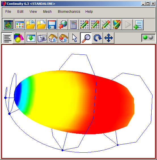
- The mesh should now look like the first screen shot
Add biomechanics data
- Load the required constitutive model from the database
- File→Library→Search…
-
In the window near the top, enter ‘lagrangian’ and hit return.
-
From the listed models select BM_TI_of_Lagrangian_strains_comp_U8_active_hilltypesympy by right-clicking on it and selecting ‘Load’
- When the warning window display, select the third choice: ‘Retain current problem but overwrite the following objects: [dims, renderer, matEquations]’
- Load the required dynamic model from the database
- File→Library→Search…
-
In the window near the top, enter ‘hilltype’ and hit return.
-
From the listed models select BM_Hilltype_sympy by right-clicking on it and selecting ‘Load’
- When the warning window display, select the third choice: ‘Retain current problem but overwrite the following objects: [dims, renderer, matEquations]’
Solve biomechanics
-
-
For Time Step, enter 2.0
-
For Number of Steps, choose 150
-
For when number of iterations >, enter 500
-
For when sum of solution increments <, enter 1e-006
-
For when sum of unconstrained residuals <, enter 1e-006
-
Click Solve, and wait for the solver to finish (do not close the Solve form!)
-
-
-
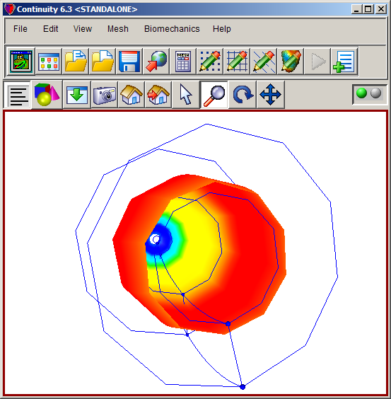
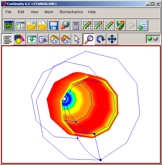
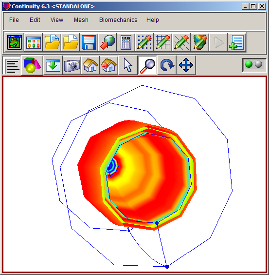
Select the deformed radio button on the bottom
-
Select the stress-out-Second Principal Invariant of C under Variables list
-
Click OK
-
Pre-built model
This cont6 file you used above for this problem already contains all data and parameters, right up to the biomechanics solve.
Animated Mesh Rendering Script
The script included with Continuity, found at pcty/examples/biomechanics01/animateHilltype.py, will run the above simulation and then animated the changes in pressure. The script can be run from within Continuity by selecting it from: File→Scripts→Read Script


