Contents
Description
- These step-by-step instructions will guide you through fitting a more complicate data set in 3D space
- The data set is obtained from 4 long-axis slices of left ventricle
- Initial truncated elipsoidal geometry is created in order to fit with the data set
- An automated script that runs this tutorial up to the point of changing to 3D is included in the Continuity installation: examples\data07\fittingLeftVentricle.py. To run it, click File→Scripts→Read script…
Start Continuity
- Launch the Continuity Client
-
On the About Continuity startup screen
-
check the fitting box under Use Modules:
-
-
Click OK to bring up the main window
Setup intial mesh
-
-
Select prolate spheriodal in the Global Coordinates: pop-up menu4
-
Enter 3.75 next to the Focus Position field
-
Click OK to submit Coordinate Form
-
-
-
Choose Lagrange Basis Function→2D→Linear-Linear
-
Click Add Linear-Linear
-
Choose Hermite Basis Function→2D→Cubic-Cubic
-
Click Add Cubic-Cubic
- Verify that the list of basis functions now contains:
- Linear-Linear Lagrange 3*3*
- Cubic-Cubic Hermite 3*3
-
Click OK to submit Basis Form
-
-
-
Click Import/Export/Graph button to open Continuity Table Manager
-
Continuity Table Manager→File→Open…
-
Select tab-delimited nodes file ( nodes.xls )
-
-
- You should now have nodes numbered 1-40
-
Select Cubic-Cubic Hermite under Coordinate 1, Coordinate 2 and under Coordinate 3
-
Click OK to submit Node Form
-
-
-
Click Import/Export button to open Continuity Table Manager
-
Continuity Table Manager→File→Open…
-
Select tab-delimited elements file ( elems.xls )
-
-
- You should now elements numbered 1-32 in the list
-
Click OK to submit Element Form
-
-
If the Fitting menu is not loaded, select File→Load Continuity Modules…
-
Select fitting and click OK
- The menu bar should now show the Fitting command
-
-
-
Click Import/Export/Graph button to open Continuity Table Manager
-
Continuity Table Manager→File→Open…
-
Select tab-delimited data file ( data.xls )
-
-
- You should now have Data numbered 1-686 in the list
-
Click OK to submit Data Form
-
-
- For all three coordinates, fill in the values according to the table below (use these as a starting guide)
s(1)
s(1)s(1)
s(2)
s(1)(2)
s(2)(2)
s(3)
s(1)s(3)
s(2)s(3)
s(3)s(3)
0.5
0.5
0.01
0.02
0.01
0.0
0.0
0.0
0.0
- For all three coordinates, fill in the values according to the table below (use these as a starting guide)
-
-
Click Import/Export/Graph button to open Continuity Table Manager
-
Continuity Table Manager→File→Open…
-
Select tab-delimited data file ( constraints.xls )
-
-
-
Click OK to submit Data Constraints Form
-
-
-
Click the lines radio button
-
Click Render
-
-
-
Click OK
-
-
-
Click on datapoints2 in the list on the left
-
Go to the Properties tab
-
Drag the Quality value to 4
-
Close the window by click the X button
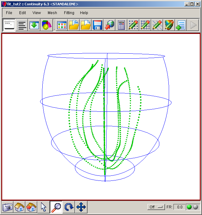
- The mesh should now look similar to the first screenshot
-
Fit prolate in lambda
-
-
In the Cooridinates tab, select coord_1, coord_2, coord_3 for the three coordinates
-
In the Xi Projections tab, enter 1-343 for Data list and 1-16 for Use points in element list
-
In the Fitting Variables tab, deselect all three coordinates
-
Click the Fit button on the bottom
-
Go back to the Xi Projections tab. Enter 344-686 for Data list and 17-32 for Use points in element list
-
Go back to the Fitting Variables tab and againdeselect all three coordinates
-
Click the Fit button on the bottom again
-
In the Fitting Variables tab, select only Coordinate 1
-
Click the Fit button one more time
-
Close the window by click the X button
-
-
-
Click the lines radio button
-
Click Render
-
-
-
Click on elements lines3 in the list on the left
-
Click on the Colors tab
-
Change the R,G,B color field to 1, 0, 0 to change the color to the brightest red and then hit Enter
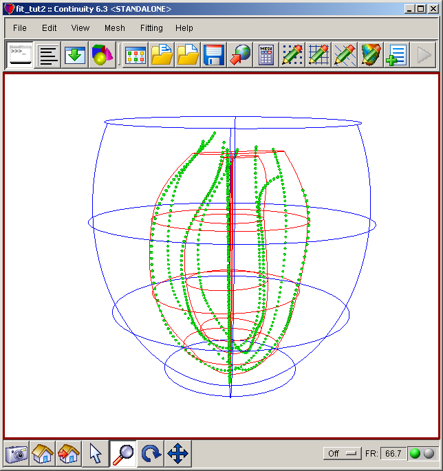
- The mesh should now look similar to the second screenshot
-
Convert to 3D
-
-
Click Import/Export button to open Continuity Table Manager
-
Continuity Table Manager→File→Open…
-
Select the second tab-delimited elements file ( elems2.xls )
-
-
- You should now have elements 1-16 in the list
-
Click OK to submit Element Form
-
-
-
Remove the two basis functions currently in the list by selecting each and then clicking the Subtract button.
-
Choose Hermite Basis Function→3D→Cubic-Cubic-Linear
-
Click Add Cubic-Cubic-Linear
-
Choose Hermite Basis Function→3D→Cubic-Cubic-Cubic
-
Click Add Cubic-Cubic-Cubic
-
Choose Lagrange Basis Function→3D→Linear-Linear-Linear
-
Click Add Linear-Linear-Linear
- Verify that the list of basis functions now contains:
- Cubic-Cubic-Linear Hermite 3*3*3
- Cubic-Cubic Hermite 3*3
- Cubic-Linear Hermite 3*3
- Linear-Cubic Hermite 3*3
- Cubic-Cubic-Cubic Hermite 3*3*3
- Linear-Linear-Linear Lagrange 3*3*3
- Linear-Linear Lagrange 3*3
-
Click OK to submit Basis Form
-
-
-
Select Cubic-Cubic-Linear under Coordinate 1
-
Select Linear-Linear-Linear under Coordinate 2 and Coordinate 3
-
Select Cubic-Cubic-Linear under Field Variable 1 in the Field Vector 1 tab
-
Click OK to submit Node Form
-
-
-
Enter 1 for xi1, 1 for xi2, and 1 for xi3 under New Element per old element in
-
Click OK to submit
-
-
-
Select Cubic-Cubic-Cubic under Coordinate 1, Coordinate 2, and Coordinate 3
-
Select Cubic-Cubic-Cubic under Field Variable 1 in the Field Vector 1 tab
-
Click OK to submit Node Form
-
-
-
Click lines radio button
-
Click Render to display mesh
-
-
-
Click on elements lines4 in the list on the left
-
Click on the Colors tab
-
Change the R,G,B color field to 0, 0.5, 0.5 to change the color to the brightest red and then hit Enter
-
Close the window by click the X button
-
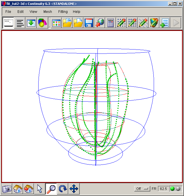
- The mesh should now look similar to the third screenshot
Pre-built model
This cont6 file contains all data and parameters for this problem prior to changing it to 3D: fit2_a.cont6 This cont6 file contains all data and parameters for this problem after changing to 3D: fit2_b.cont6 The model is also loaded into the Continuity database (ID: 1303) with run scripts in the script manager.


