Inflation of a Passive Left Ventricular Model With Infarct

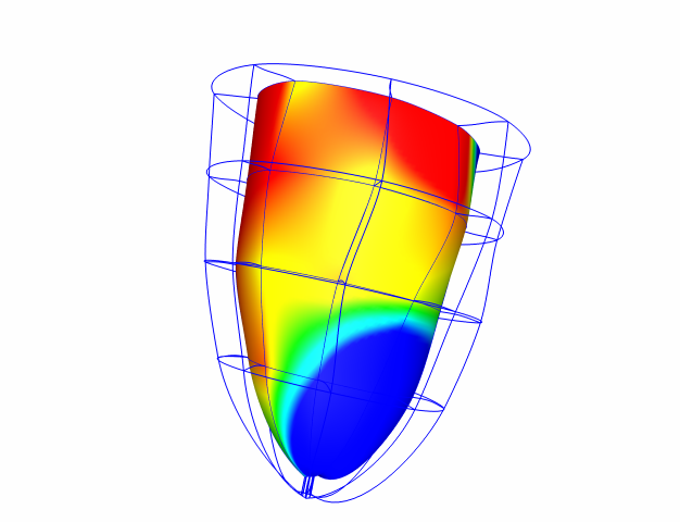
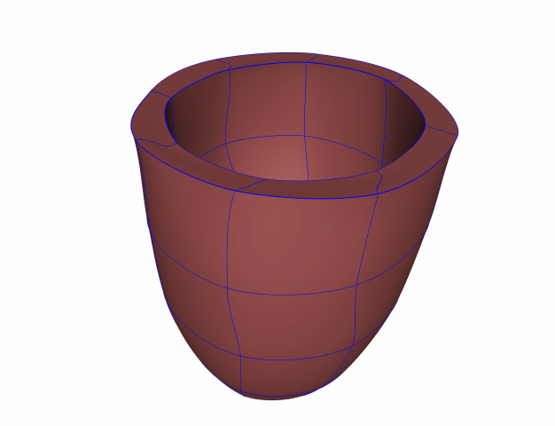
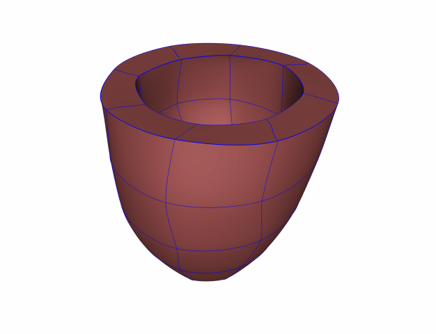
Description

• This example guides you through setting up and running a physical and material nonlinear problem of the passive inflation of a left ventricular model using pressure (natural) boundary conditions.
• The mesh consists of 48 tri-cubic (cubic-cubic-cubic) elements. The material chosen is a transversely isotropic exponential strain energy function. The material is stiffer in the fiber direction than perpendicular to them. The fibers whose orientation is defined by fiber angles in the node form with respect to the circumferential direction vary linearly in radial direction across the wall from -60 degrees on the epicardium to +60 degrees on the endocardium. The boundary conditions assure that all rigid body motions are suppressed. Pressure is prescribed on the endocardium to simulate the passive filling of a ventricle (diastole).
• The model has an apical infarct. The myocardium is stiffer in the infarct region.

Start Continuity

• Launch the Continuity 6.4 Client

• On the About Continuity 6.4 startup screen

  • leave the mesh checkbox checked under Use Modules:

  • check the biomechanics checkbox under Use Modules:

• Click OK to bring up the main window

Load File From Database

Load Model

• File→Library→Search…

  • Right click on the entry Pat7_Unloaded_Inflation.

  • Click Load.

  • Choose Reset or not based on if you already have a model open.

Edit Model

• Mesh→Edit→Material Coordinates…

  • Under Parameters change the the Fiber angle from a set value of zero getting the fiber angle from a field.

  • Select the Fiber Angle field to use the predefined fiber angles.

• Mesh→Edit→Nodes…

  • In the nodes form, select a Linear-Linear-Linear basis function for Field Variable 2

• File→Send

  • If the Dimensions Form appears, simply click Apply Marked Recommendations and then OK

• Mesh→Calculate Mesh…

List Volume

• Mesh→List→Volume…

  • Select undeformed or deformed under Select a Mesh

  • Click OK to submit List Volume Form

Render Elements

• Mesh→Render→Elements…

  • Click the lines radio button

  • Click Render to display mesh lines

  • Click the surfaces or texture radio button

  • For 3D elements, chose an Xi plane (1, 2 or 3) to render

  • Enter an Xi Location between 0.0 and 1.0 for rendering the surface

  • Click Render to display mesh surfaces

Render Fibers

• Mesh→Render→Fibers…

  • Specify a list of Elements to render or leave the default all

  • Specify a list of Xi3 Locations

  • Specify a vector Length normalized by the element dimension or click Auto

  • Specify the number of material vectors to render per element in each direction

  • Click OK to render material axes

Biomechanics Menu

Edit Constitutive Model

• Biomechanics→Edit→Constitutive Model…

• Use the Edit equations tab to create and name intermediate symbolic or evaluated variables and write the equations that define the Dependent variable for this model, which is Stress in terms of the Independent variableswhich include hydrostatic pressure, the material coordinate transformation dY_dMatl, the deformation gradient of deformed curvilinear coordinate with respect to undeformed material coordinates dX_dMatl, and the curvilinear world coordinate transformation dy_dx.

  • Stress is a square matrix containing the components of the Lagrangian Second Piola-Kirchhoff Stress tensor with respect to material coordinates.

  • Equations are entered using Sympy

• Use the Parameters list to set adjustable material parameters

  • The model Parameters list is generated from the equations. Quantities delimited by <anglebrackets> in the equations are parameters

  • Select a parameter in the list

    • You can edit its Description, specify its default value to be defined by a constant value or a field variable or a field variable derivative.

    • You can also add exceptions using the Add exception in… popup menu that allows alternative parameter values or fields to be specified according to a prescribed element list or a prescribed field range for a specified field variable.

• The View equations displays a complete listing of the Sympy equations defining the model.

• The Compile button is where C code is generated from the Sympy model and compiled

  • Click the Compile button to compile the model on the default server

  • Click View code to generate and view a C code listing of the model

• Click the Submit button in the Submit tab to submit the Constitutive Model.

Edit Boundary Conditions

• Biomechanics→Edit→Boundary Conditions…

  • The Initial Conditions tab looks like the Coordinates tab of the Mesh→Edit→Nodes… form.

  • You can use the Biomechanics→Update→Initial conditions with undeformed nodes command to initialize the Deformed Coordinates with the undeformed nodal coordinates.

  • Use the tabs Deformed Coordinate 1, Deformed Coordinate 2, Deformed Coordinate 3, Hydrostatic Pressure to specify nodal boundary conditions

    • Click Insert Nodes to create a boundary condition for one or more nodes.

    • Insert a node number, list of node numbers or node number label in the Node(s) field

    • Use the pop-up menu to choose a nodal Derivative parameter to constrain or apply force to

    • Use the pop-up menu to select displacement, force, coupled or spring Boundary Condition Type

    • Enter a value where 0.0 would mean no displacement or force

    • If coupled Boundary Condition Type is selected, the second row of options is enabled

      • You can couple the specified constrained nodal degrees of freedom to a selected Derivative of one or more Coupled Node(s) of a selected Dependent variable via a coupling Coefficient. Enter one or more Coupled Node(s), select Derivative and Dependent Variable from the appropriate pop-pu menus and enter the coupling Coefficient

  • Click the OK button to submit Boundary Conditions Form

Update Initial conditions with undeformed nodes

• Biomechanics→Update→Initial conditions with undeformed nodes

  • This command copies the nodal geometric coordinates and derivatives from the Node Form to the Initial Conditions tab of the Boundary Conditions Form

Solve Nonlinear

• Biomechanics→Solve Nonlinear…

  • Specify the Time Step as 0.0, Initial Time as 1.0, and Number of Steps as 10

  • Click the Solve button, and wait for the solver to finish. While the solution is being computed the window will remain open. There will also be output listed to the console window and the Python shell.

List Stress and Strain

• Biomechanics→List Stress and Strain…

  • In the Variables tab, use checkboxes to deselect any variables you do not wish to list

  • Note that the Output Variables are calculated using the equations entered in the Output Variable folder of the submitted Constitutive model

  • In the Locations tab, you can selected the element list and points which which solutions will be listed

  • Click OK to display a listing of the selected Output Variables in the Table Manager

Render Surface

• Biomechanics→Render Surface…

  • Enter Element List or leave default value or all

  • Select an unused Field Variable that will hold nodal values of the solution to be interpolated and rendered

  • Check the undeformed or deformed radio button to indicate whether you want to the solution rendered on the undeformed or deformed geometry

  • Select the output variable form the menu. For vector and tensor variables, a choice of components will be presented. Output will be referred to coordinate frames as determined by equations in the Output Variablesfolder of the Constitutive Model Editor

  • Click OK to create a color-coded surface rendering of the chosen output variable